Tuesday, January 30, 2018

How to Update a Column based on Count of repeated Items in another Column in SQL Server

SQL Query to Update a Column based on Count of repeated Items in another Column
Scenario:
Suppose we have a table as follows
SELECT [Order_Id]
      ,[Geo_Id]
      ,[Cust_Name]
      ,[Sales_Region]
      ,[Deal_Id]
      ,[Net_Sales]
  FROM [dbo].[tbl_Sample]
GO


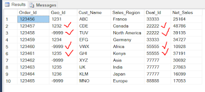
In this Table , we have to update the Column Geo_Id based on the following Conditions :
A). If we have only 2 Geo_Ids, one =-9999 and Other one <> -9999 ( Eg: -9999 , 1232 ) under the same Deal_Id ( Eg : 22222) Then we need to update the Geo_Id "-9999" with another Geo_Id , say 1232.
B). If we have only one Geo_Id , as -9999 under a Deal_Id ( Eg: 88888) then we should not perform any update.
C). If we have more than two Geo_Ids , one =-9999 and Others<> -9999  (Eg : -9999,1235 1236 ) under the same Deal_Id ( Eg : 77777) then we should not perform any update.

Now we can achieve this Scenario using the below Methods :

1) Sub Query Method :
Update [tbl_Sample]
Set  Geo_Id =S1.Geo_ID
From (
SELECT A.Order_Id,A.Geo_Id,A.Cust_Name,A.Sales_Region,B.Deal_Id,                                             A.Net_Sales,B.GeoCountByDeal
FROM [tbl_Sample] A
Inner Join (
SELECT COUNT(Distinct Geo_Id) as GeoCountByDeal, B.Deal_Id
         FROM [tbl_Sample] B
 GROUP BY B.Deal_Id
AS B 
    ON A.Deal_Id = B.Deal_Id
   WHERE GeoCountByDeal=2 and A.Geo_Id<>'-9999' 
   -- ORDER by A.Deal_Id
) S1
Where ( [tbl_Sample].Deal_Id=S1.Deal_Id and [tbl_Sample].Geo_Id=-9999 and S1.GeoCountByDeal=2 )
Select * From [tbl_Sample]
GO

2) Common Table Expressions (CTEs) Method :
WITH MyCTE
AS
(
SELECT A.Order_Id,A.Geo_Id,A.Cust_Name,A.Sales_Region,B.Deal_Id,                                             A.Net_Sales,B.GeoCountByDeal
FROM [tbl_Sample] A
Inner Join (
SELECT COUNT(Distinct Geo_Id) as GeoCountByDeal, B.Deal_Id
         FROM [tbl_Sample] B
 GROUP BY B.Deal_Id
AS B 
    ON A.Deal_Id = B.Deal_Id
   WHERE GeoCountByDeal=2 and A.Geo_Id<>'-9999' 
   -- ORDER by A.Deal_Id

Update [tbl_Sample]
Set  [tbl_Sample].Geo_Id =MyCTE.Geo_ID
From MyCTE
Where ( [tbl_Sample].Deal_Id=MyCTE.Deal_Id and [tbl_Sample].Geo_Id=-9999 and MyCTE.GeoCountByDeal=2 )
Select * From [tbl_Sample]
;
GO

Output after Update:


--------------------------------------------------------------------------------------------------------
Thanks, TAMATAM ; Business Intelligence & Analytics Professional
-------------------------------------------------------------------------------------------------------
-

Sunday, January 28, 2018

What is Data Frame and How to Create a Data Set in R Programming

The Data Frame in R Programming
A data frame is a Table or a two dimensional array like structure in which each column contains the values of same mode and each row contains the same set of values from each column.
The data frame is a structure in R that holds data and is similar to the datasets found in the standard statistical packages (for example, SAS, SPSS, and Stata). The columns are  the variables, and the rows are observations. You can have variables of different types (numeric or character, logical) with each column having same type/mode of data in the data frame. Data frames are the main structures you use to store datasets.

Characteristics of Data frame :
--The column names should not be empty
--The row names should be unique.
--The data stored in the data frame can be of numeric, factor, or character type.
--Each column should have the same mode of data and same number of data items.

Creating a Data frame :
> emp_id<-c(1:5)
> emp_name<-c("Rick","Dan","Michelle","Ryan","Gary")
> salary<-c(624.53,515.25,615.10,725.45,845.25)
> start_date<-as.Date(c("2012-01-01","2013-09-23","2014-11-15","2014-05-11","2015-03-27"))

> empdata<-data.frame(emp_id,emp_name,salary,start_date,stringsAsFactors = FALSE)
> head(empdata) # same as  print(empdata)
   emp_id emp_name    salary    start_date
1     1             Rick        624.53   2012-01-01
2     2             Dan         515.25   2013-09-23
3     3            Michelle   615.10   2014-11-15
4     4            Ryan        725.45   2014-05-11
5     5            Gary        845.25    2015-03-27


#Getting the Structure of the Data frame :
> str(empdata)
'data.frame': 5 obs. of 4 variables:
$ emp_id : int 1 2 3 4 5
$ emp_name : chr "Rick" "Dan" "Michelle" "Ryan" ...
$ salary : num 625 515 615 725 845
$ start_date: Date, format: "2012-01-01" "2013-09-23" "2014-11-15" "2014-05-11" ...

#Summary of data in the Data frame :
The statistical summary and nature of the data can be obtained by applying the summary() function.
> summary(empdata)
emp_id       emp_name               salary                start_date
Min.     :  1   Length:5                 Min.   :515.2       Min.    : 2012-01-01
1st Qu.:  2   Class :character     1st Qu.:615.1     1st Qu.: 2013-09-23
Median:  3   Mode  :character    Median :624.5    Median: 2014-05-11
Mean   :  3                                  Mean   :665.1    Mean   : 2014-01-14
3rd Qu.:  4                                  3rd Qu.:725.5    3rd Qu.: 2014-11-15
Max.   :   5                                   Max.   :845.2     Max.    : 2015-03-27 

Extracting data from a Data frame :
We can extract the specific columns data from a data frame using column names as follows. 
> result<-data.frame(empdata$emp_name,empdata$salary)
> result
       empdata.emp_name   empdata.salary
1               Rick                         624.53
2               Dan                         515.25
3               Michelle                   615.10
4               Ryan                       725.45
5               Gary                        845.25

> class(result)
[1] "data.frame"
here, result is another data frame formed from the data frame empdata

#Extracting first 2 observations(rows) from a Data frame :
> result<-emp.data[1:2,]
> result
   emp_id emp_name    salary    start_date
1     1             Rick        624.53   2012-01-01
2     2             Dan         515.25   2013-09-23

#Extracting data from 3rd , 5th rows and 2nd,4th columns of a Data frame :
> result<-empdata[c(3,5),c(2,4)]

> result
       emp_name     start_date
3       Michelle       2014-11-15
5       Gary            2015-03-27

Adding new Columns and Rows to a Data frame :
A data frame can be expanded by adding rows and columns to it.
# Adding the "dept" column to the above data frame
> empdata$dept<-c("IT","Operations","IT","HR","Finance")
>print(empdata)
   emp_id emp_name    salary    start_date     dept
1     1             Rick        624.53   2012-01-01     IT
2     2             Dan         515.25   2013-09-23    Operations
3     3            Michelle   615.10   2014-11-15     IT
4     4            Ryan        725.45   2014-05-11     HR
5     5            Gary        845.25    2015-03-27    Finance


# To combine a one row to the above data frame
We can combine a row to the Data frame using the rbind() function, which will forms a new data frame with additional row.
> newdata<-rbind(empdata,list(6, "Laura",985.75,"2015-08-15","HR"))

#Adding the new rows to the above data frame
To add more rows permanently to an existing data frame, we need to bring the new rows in the same structure as the existing data frame and then use rbind () function.
Here in the below example we create a new data frame with new rows and then merge with the existing data frame to create the final data frame.

# Creating a new data frame
> emp_id<-c(6:8)
> emp_name<-c("Shreya","Ravi","Teja")
> salary<-c(575.53,725.15,635.10)
> start_date<-as.Date(c("2013-05-25","2013-07-30","2014-06-15"))
> dept<-c("F&A","BI","R&D")
> empnewdata<-data.frame(emp_id,emp_name,salary,start_date,dept,stringsAsFactors = FALSE)
> empnewdata

  emp_id   emp_name salary    start_date     dept
1      6        Shreya       575.53   2013-05-25  F&A
2      7        Ravi           725.15   2013-07-30   BI
3      8        Teja           635.10    2014-06-15  R&D

# Bind or combining the new data frame with existing one
> empfinaldata<-rbind(empdata,empnewdata)
> empfinaldata
   emp_id emp_name    salary    start_date     dept
1     1             Rick        624.53   2012-01-01     IT
2     2             Dan         515.25   2013-09-23    Operations
3     3            Michelle   615.10   2014-11-15     IT
4     4            Ryan        725.45   2014-05-11     HR
5     5            Gary         845.25   2015-03-27    Finance
6     6            Shreya     575.53   2013-05-25    F&A
7     7            Ravi         725.15   2013-07-30    BI
8     8            Teja          635.10   2014-06-15    R&D


Thanks, Tamatam

What are the Factors and How to Create them in R Programming

The Factors in R Programming
Factors are the data Objects which are used to categorize the data and store it as levels.They can store both strings and integers.They are useful in the Columns which have limited no.of unique values, like "Male", "FeMale" , and "True", "False" etc.

Categorical (nominal) and ordered categorical (ordinal) variables in R are called factors. The Factors are crucial in R because they determine how data is analyzed and presented visually.


As you’ve seen, variables can be described as nominal, ordinal, or continuous. Nominal
variables are categorical
, without an implied order. Diabetes (Type1, Type2) is an example of a nominal variable. Even if Type1 is coded as a 1 and Type2 is coded as a 2 in the data, no order is implied

Ordinal variables imply order but not amount. Status (poor, improved, excellent) is a good example of an ordinal variable. We know that a patient with a poor status isn’t doing as well as a patient with an improved status, but not by how much.

Continuous variables can take on any value within some range,and both order and amount are implied. Age in years is a continuous variable and can take on values such as 14.5 or 22.8 and any value in between. You know that someone who is 15 is one year older than someone who is 14.

Factors are created using the the Factor() function by taking vector as input.

Create a Factor:
# Creating a vector as input
> data<-c("East","West","East","North","North","East","West","West","West","East","North")

> print(data)
 [1] "East"  "West"  "East"  "North" "North" "East"  "West"  "West"  "West"  "East"  "North"

> print(is.factor(data))
[1] FALSE

# Creating a Factor with above vector as input with factor() function
> factor_data<-factor(data)
> print(factor_data)
 [1] East  West  East  North North East  West  West  West  East  North
Levels: East North West
> print(is.factor(factor_data))
[1] TRUE

Factors in Data Frame:
On creating any data frame (dataset) with a column of text data , R treats the text column as categorical data and creates the factors on it.
# Creating the vectors for a data frame
> height<-c(132,151,162,139,166,147,122)
> weight<-c(48,49,66,53,67,52,40)
> gender<-c("male","male","female","female","male","female","male")


Creating the data frame from above vectors
> input_data<-data.frame(height,weight,gender)
> print(input_data)
  height weight gender
1    132     48   male
2    151     49   male
3    162     66 female
4    139     53 female
5    166     67   male
6    147     52 female
7    122     40   male

Test the which column is a factor
> print(is.factor(input_data$height))
[1] FALSE
> print(is.factor(input_data$weight))
[1] FALSE

> print(is.factor(input_data$gender))
[1] TRUE

Print the gender column to see the factor levels
> print(input_data$gender)

[1] male   male   female female male   female male  

Levels: female male

Changing the Order of Levels in Factor:
# Creating a Factor with above vector as input with factor() function
> data<-c("East","West","East","North","North","East","West","West","West","East","North")
> factor_data<-factor(data)
> print(factor_data)
 [1] East  West  East  North North East  West  West  West  East  North
Levels: East North West
By default the order of the Levels are shown in Alphabetical (a,b,c..) order. We can also change the order as we wish by specifying the levels in factor as shown below.
> new_order_data<-factor( factor_data, levels=c("East","West","North"))
> new_order_data
 [1] East  West  East  North North East  West  West  West  East  North
Levels: East West North

Generating Factor Levels:
We can generate the Factor levels by using the gl() function. It takes two integers (n,k) as input, where n indicates the no.of levels and k indicates the no.of times each level should replicate(repeat).

syntax:
gl(n,k, labels)

here,n indicates the no.of levels and k indicates the no.of times each level should replicate and labels is a vector of labels for the resulting factor levels.

> v<-gl(3,4,labels=c("East","West","North"))
> v
 [1] East  East  East  East  West  West  West  West  North North North North
Levels: East West North

Nominal vs Ordinal Factors :
The function factor() stores the categorical values as a vector of integers in the range [1… k], (where k is the number of unique values in the nominal variable) and an internal vector of character strings (the original values) mapped to these integers.
For example, assume that we have this vector:
>diabetes <- c("Type1", "Type2", "Type1", "Type1")

> diabetes
[1] "Type1" "Type2" "Type1" "Type1"
> diabetes <- factor(diabetes)
> diabetes

[1] Type1 Type2 Type1 Type1

Levels: Type1 Type2

The statement diabetes <- factor(diabetes) stores this vector as (1, 2, 1, 1) and associates it with 1 = Type1 and 2 = Type2 internally (the assignment is alphabetical).
Any analyses performed on the vector diabetes will treat the variable as nominal and select the statistical methods appropriate for this level of measurement.

For vectors representing ordinal variables, you add the parameter ordered=TRUE to the factor() function.
>status <- c("Poor", "Improved", "Excellent", "Poor")
>status <- factor(status, ordered=TRUE)
>status

[1] Poor      Improved  Excellent Poor     

Levels: Excellent < Improved < Poor
The statement status <- factor(status, ordered=TRUE) will encode the vector as (3, 2, 1, 3) and associate these values internally as 1 = Excellent, 2 = Improved, and 3 =Poor. Additionally, any analyses performed on this vector will treat the variable as ordinal and select the statistical methods appropriately.

By default, factor levels for character vectors are created in alphabetical order. This worked for the status factor, because the order “Excellent,” “Improved,” “Poor” made sense. 

There would have been a problem if “Poor” had been coded as “Average” instead, because the order would have been “Average,” “Excellent,” “Improved.” A similar problem would exist if the desired order was “Poor,” “Improved,” “Excellent.” 

For ordered factors, the alphabetical default is rarely sufficient.You can override the default by specifying a levels option. 
Example:
> status <- factor(status, order=TRUE, levels=c("Poor", "Improved", "Excellent"))

> status
[1] Poor      Improved  Excellent Poor
Levels: Poor < Improved < Excellent

The above statement assigns the levels as 1 = Poor, 2 = Improved, 3 = Excellent. Be sure the specified levels match your actual data values. Any data values not in the list will be set to missing.

Numeric variables can be coded as factors using the levels and labels options. If the gender was coded as 1 for male and 2 for female in the original data, then
>gender<-c(1,2)
> gender<- factor(gender)
> gender
[1] 1 2
Levels: 1 2
>gender<- factor(gender, levels=c(1, 2), labels=c("Male", "Female")) would convert the variable to an un ordered factor.
>gender
[1] Male   Female
Levels: Male Female

Note that the order of the labels must match the order of the levels. In this example, gender would be treated as categorical,the labels “Male” and “Female” would appear in the output instead of 1 and 2, and any gender value that wasn’t initially coded as a 1 or 2 would be set to missing.

Example :
The following listing demonstrates how specifying factors and ordered factors impacts data analyses.
First we enter the data as vectors. Then you specify that diabetes is a factor and status is an ordered factor. Finally, you combine the data into a data frame. 
> patientID <- c(1, 2, 3, 4)
> age <- c(25, 34, 28, 52)
> diabetes <- c("Type1", "Type2", "Type1", "Type1")
> status <- c("Poor", "Improved", "Excellent", "Poor")
> diabetes <- factor(diabetes)
> status <- factor(status, order=TRUE)

> patientdata <- data.frame(patientID, age, diabetes, status)
> str(patientdata)
‘data.frame’: 4 obs. of 4 variables:
$ patientID: num 1 2 3 4
$ age : num 25 34 28 52
$ diabetes : Factor w/ 2 levels "Type1","Type2": 1 2 1 1
$ status : Ord.factor w/ 3 levels "Excellent"<"Improved"<..: 3 2 1 3

> summary(patientdata)

patientID age diabetes status
Min. :1.00 Min. :25.00 Type1:3 Excellent:1
1st Qu.:1.75 1st Qu.:27.25 Type2:1 Improved :1
Median :2.50 Median :31.00 Poor :2
Mean :2.50 Mean :34.75
3rd Qu.:3.25 3rd Qu.:38.50
Max. :4.00 Max. :52.00


Notes :
The function str(object) provides information about an object(here, the data frame) in R .It clearly shows that diabetes is a factor and status is an ordered factor, along with how they are coded internally. 

Note that the summary() function treats the variables differently. It provides the minimum, maximum, mean, and quartiles for the continuous variable age, and frequency counts for the categorical variables diabetes and status.


Thanks, TAMATAM

Saturday, January 27, 2018

What is List Indexing and How to Access,Add and Delete the List Elements in R Programming

General List Operations in R Programming
We perform various List Operations like List Indexing, Adding, Deleting List elements and accessing the List elements.
Consider the following example of list, based on which we perform some general operations
j <- list(name="Joe", salary=55000, unionms=T)
> j
$name
[1] "Joe"
$salary
[1] 55000
$unionms
[1] TRUE

1) List Indexing :
You can access a list components/elements in 3 different ways:
> j$salary
[1] 55000

> j[["salary"]]
[1] 55000

> j[[2]]
[1] 55000

We can refer to list components by their numerical indices, treating the list as a vector. However, note that in this case, we use double brackets instead of single ones.
So, there are three ways to access an individual component c of a list Lst and return it in the data type of c


Lst $cLst [["c"]]
Lst [[i]]                # here i is the index of c within Lst

An alternative to the second and third techniques listed is to use single brackets rather than double brackets:


Lst["c"]
Lst[i]                  # here i is the index of c within Lst


Both single-bracket and double-bracket indexing access list elements in vector-index way. But there is an important difference from ordinary (atomic) vector indexing.If single brackets [ ] are used, the result is another list--a sublist of the original. 
For instance, continuing to the preceding example, we can have this:

> j[1:2]
$name
[1] "Joe"
$salary
[1] 55000

> j2 <- j[2]
> j2

$salary
[1] 55000

> class(j2)
[1] "list"
> str(j2)
List of 1
$ salary: num 55000


Note:
The subsetting operation returned another list consisting of the first two components of the original list j. Note that the word returned makes sense here, since index brackets are functions. This is similar to other cases we’ve seen for operators that do not at first appear to be functions, such as +.
We can use double brackets [[ ]] for referencing only a single component, with the result having the type of that component.

> j[[1:2]]
Error in j[[1:2]] : subscript out of bounds

> j2a <- j[[2]]
> j2a
[1] 55000

> class(j2a)
[1] "numeric"

2) Adding and Deleting List Elements :
We can add and delete the list elements. The new components can be added after a list is created.
> z <- list(a="abc",b=12)
> z
$a
[1] "abc"

$b
[1] 12


# adding a c component to the existing list
> z$c <- "third"
> z
$a
[1] "abc"
$b
[1] 12
$c
[1] "
third"

We can also add components via a vector index:
> z[[4]] <- 28
> z[5:7] <- c(FALSE,TRUE,TRUE)


> z
$a
[1] "abc"
$b
[1] 12
$c
[1] "
third"

[[4]]
[1] 28
[[5]]
[1] FALSE
[[6]]
[1] TRUE
[[7]]
[1] TRUE

We can delete a list component by setting it to NULL.
> z$b <- NULL
> z$a
[1] "abc"
$c
[1] "
third"
[[3]]
[1] 28
[[4]]
[1] FALSE
[[5]]
[1] TRUE
[[6]]
[1] TRUE

Note:
Note that upon deleting z$b, the indices of the elements after it moved up by 1. For instance , the above z[[4]] became z[[3]].

We can also concatenate lists as follows :
z<-c(list("Joe", 55000, T),list(5))

[[1]]
[1] "Joe"
[[2]]
[1] 55000
[[3]]
[1] TRUE
[[4]]
[1] 5

Getting the Size of a List
Since a list is a vector, you can obtain the number of components in a list via length().
> length(z)
[1] 4

3) Accessing List Components and Values :
Consider the following list
j <- list(name="Joe", salary=55000, unionms=T)
> j
$name
[1] "Joe"
$salary
[1] 55000
$unionms
[1] TRUE

If the components in a list do have tags, as is the case with name, salary, and unionms for j , you can obtain them via names().
The return value of unlist() is a vector—in this case, a vector of character strings. Note that the element names in this vector come from the components in the original list.
> names(j)
[1] "name" "salary" "unionms"


To obtain the values, use unlist():

> ulj <- unlist(j)
> ulj
name salary unionms
"Joe" "55000" "TRUE"
> class(ulj)
[1] "character"

On the other hand, if we were to start with numbers, we would get numbers.The output of unlist() in this case was a numeric vector.
> z <- list(a=5,b=12,c=13)
> y <- unlist(z)

> class(y)
[1] "numeric"
> y
a b c
5 12 13


In case of Mixed mode of data, how unlist() will works is shown below example;
> w <- list(a=5,b="xyz")
> wu <- unlist(w)
> class(wu)
[1] "character"

> wu
  a   b
"5" "xyz"

Note:
Where possible the list components are coerced to a common mode during the unlisting, and so the result often ends up as a character vector. Vectors will be coerced to the highest type of the components in the hierarchy NULL < raw < logical < integer < real < complex < character < list < expression: pair lists are treated as lists.

Removing the List element Names :
In the above example,though wu is a vector and not a list, R did give each of the elements a name. We can remove them by setting their names to NULL.
> names(wu) <- NULL
> wu
[1] "5" "xyz"

We can also remove the elements’ names directly with unname(), as follows:
> wun <- unname(wu)
> wun
[1] "5" "xyz"


4) Using the lapply() and sapply() Functions on Lists:
The function lapply() (for list apply) works like the matrix apply() function,calling the specified function on each component of a list (or vector coerced to a list) and returning another list. Here’s an example, where R applied median() to 1:3 and to 25:29, returning a list consisting of 2 and 27.
>lapply(list(1:3,25:29),median)
[[1]]
[1] 2


[[2]]
[1] 27

Note:
In some cases, such as the example here, the list returned by lapply() could be simplified to a vector or matrix. This is exactly what sapply() (for simplified [l]apply) does.
> sapply(list(1:3,25:29),median)
[1] 2 27

Thanks, TAMATAM

What is List and How to Create it in R Programming

The Lists in R Programming
A list is an ordered collection of objects (components). Lists are referred to as the recursive vectors. In a list we can store different modes or types of data.
A list allows you to gather a variety of (possibly unrelated) objects under one name. A list may contain a combination of vectors,matrices, data frames, and even other lists.

Lists are important R structures for two reasons. First,they allow you to organize and recall disparate information in a simple way. Second,the results of many R functions return lists. 

Creating a List :

We create a list using the list() function
mylist <- list(object1, object2, ...)
here the objects are any of the structures (
vectors,matrices..). Optionally, you can name the objects in a list:
mylist <- list(name1=object1, name2=object2, ...)

Example 1:
let’s consider an employee database. For each employee, we wish to store the name, salary , and a Boolean indicating union membership. Since we have three different modes here—character, numeric,and logical. So that we can use the list here to store different modes of this data.

We could create a list to represent our employee, Joe, this way:
j<- list(name="Joe", salary=55000, unionms=T)

#The result of the list displays all its components

> j
$name
[1] "Joe"
$salary
[1] 55000
$unionms
[1] TRUE

Also we can create the list without specifying the object names.
j<- list("Joe",55000,T)
>j
[[1]]
[1] "Joe"
[[2]]
[1] 55000
[[3]]
[1] TRUE

It could be ideal to use the names instead of numeric indices.
We can access the specific object of a list as follows..


> j$sal
[1] 55000

Since Lists are also a kind of vectors, they can be created via vector():
> z <- vector(mode="list")
> z[["abc"]] <- 3
> z
$abc
[1] 3

Example 2:
In this example, you create a list with four components: a string, a numeric vector, a matrix, and a character vector. You can combine any number of objects and save them as a list.
> g <- "My Sample List"

> h <- c(25, 26, 18, 39)
> j <- matrix(1:10, nrow=5)
> k <- c("one", "two", "three")
> mylist <- list(title=g, ages=h, j, k)

> mylist
$title
[1] "My Sample List"

$ages
[1] 25 26 18 39

[[3]]
     [,1] [,2]
[1,]  1   6
[2,]  2   7
[3,]  3   8
[4,]  4   9
[5,]  5  10

[[4]]
[1] "one" "two" "three"

You can also specify elements of the list by indicating a component number or a name within double brackets. In this example, mylist[[2]] and mylist[["ages"]] both refer to the same four-element numeric vector. For named components,mylist$ages would also work.

> mylist[[2]]
[1] 25 26 18 39

> mylist[["ages"]]
[[1] 25 26 18 39

Notes:
The period (.) has no special significance in object names. The dollar sign ($) has a some what analogous meaning to the period in other object-oriented languages and can be used to identify the parts of a data frame or list. For example, A$x refers to variable x in data frame A.

R doesn’t provide multi line or block comments. You must start each line of a multi line comment with #. For debugging purposes, you can also surround code that you want the interpreter to ignore with the statement if(FALSE){...}.Changing the FALSE to TRUE allows the code to be executed.
■ Assigning a value to a nonexistent element of a vector, matrix, array, or list expands that structure to accommodate the new value. For example, consider the following:
> x <- c(8, 6, 4)
> x[7] <- 10

> x
[1] 8 6 4 NA NA NA 10


The vector x has expanded from three to seven elements through the assignment. x<- x[1:3] would shrink it back to three elements.
■ R doesn’t have scalar values. Scalars are represented as one-element vectors.
■ Indices in R start at 1, not at 0. In the vector earlier, x[1] is 8.
■ Variables can’t be declared. They come into existence on first assignment.

Thanks, TAMATAM

Featured Post from this Blog

How to compare Current Snapshot Data with Previous Snapshot in Power BI

How to Dynamically compare two Snapshots Data in Power BI Scenario: Suppose, we have a sample Sales data, which is stored with Monthly Snaps...

Popular Posts from this Blog