R is a programming language and software environment for statistical analysis, computing and graphics, similar to the S language originally developed at Bell Labs. It’s an open source solution to data analysis that’s supported by a large and active worldwide research community.

command prompt (>) or run a set of commands from a source file. There are a wide variety of data types, including vectors, matrices, data frames (similar to datasets), and lists (collections of objects).
Comments are like helping text in your R program and they are ignored by the interpreter
while executing your actual program. Single comment is written using # in the beginning of the statement as follows:
# This is the Single line Comment in R Programming
R does not support multi-line comments but you can perform a trick which is something
as follows:
R help functions :
The Workspace :
The workspace is your current R working environment and includes any user-defined objects (vectors, matrices, functions, data frames, and lists).
Packages :
R comes with extensive capabilities right out of the box. But some of its most exciting features are available as optional modules that you can download and install. There are more than 5,500 user-contributed modules called packages that you can download from http://cran.r-project.org/web/packages. They provide a tremendous range of new capabilities, from the analysis of geospatial data to protein mass spectra processing
to the analysis of psychological tests.
Packages are collections of R functions, data, and compiled code in a well-defined format.
The directory where packages are stored on your computer is called the library.
The function .libPaths() shows you where your library is located, and the function library() shows you what packages you’ve saved in your library.
R comes with a standard set of packages (including base, datasets, utils, grDevices, graphics, stats, and methods). They provide a wide range of functions and datasets that are available by default. Other packages are available for download and installation.
Once installed, they must be loaded into the session in order to be used. The command search() tells you which packages are loaded and ready to use.
Example:
The following gives an error as −1 is not a complex value.
> sqrt(−1) # square root of −1
[1] NaN
Warning message:
In sqrt(−1) : NaNs produced
Instead, we have to use the complex value −1 + 0i.
> sqrt(−1+0i) # square root of −1+0i
[1] 0+1i
An alternative is to coerce −1 into a complex value.
> sqrt(as.complex(−1))
[1] 0+1i
D) Logical:
A logical value is often created via comparison between variables.
> x <- 4; y <- 7 # sample values
> z = x > y # is x larger than y?
> z # print the logical value
[1] FALSE
> class(z) # print the class name of z
[1] "logical"
Standard logical operations are "&" (and), "|" (or), and "!" (negation).
> u <- TRUE; v <- FALSE
> u & v # u AND v
[1] FALSE
> u | v # u OR v
[1] TRUE
> !u # negation of u
[1] FALSE
Further details and related logical operations can be found in the R documentation.
> help("&")
Two character values can be concatenated with the paste function.
> fname <- "James"; lname <-"Bond"
> paste(fname, lname)
[1] "James Bond"
To extract a substring, we apply the substr function. Here is an example showing how to extract the substring between the third and twelfth positions in a string.
> substr("Mary has a little lamb.", start=3, stop=12)
[1] "ry has a l"
And to replace the first occurrence of the word "little" by another word "big" in the string, we apply the sub function.
> sub("little", "big", "Mary has a little lamb.")
[1] "Mary has a big lamb."
More functions for string manipulation can be found in the R documentation.
> help("sub")
We will discuss about each below Object in detail in upcoming tutorials.
R functionality can be integrated into applications written in other languages, iincluding C++, Java, Python, PHP, Pentaho, SAS, and SPSS. This allows you to continue working in a language that you may be familiar with, while adding R’s capabilities to your applications.
Obtaining and installing R :
R is freely available from the Comprehensive R Archive Network (CRAN) at :
R is freely available from the Comprehensive R Archive Network (CRAN) at :
Precompiled binaries are available for Linux, Mac OS X, and Windows.

R Studio :
The Tool where you develop/debug your R Programming using R Console. First you need install the R from above step then download the R Studio from the below R Studio link to work on it:

> q() function Quits R. You’ll be
prompted to save the workspace.
Working with R :
R is a case-sensitive, interpreted language. You can enter commands one at a time at thecommand prompt (>) or run a set of commands from a source file. There are a wide variety of data types, including vectors, matrices, data frames (similar to datasets), and lists (collections of objects).
Comments are like helping text in your R program and they are ignored by the interpreter
while executing your actual program. Single comment is written using # in the beginning of the statement as follows:
# This is the Single line Comment in R Programming
R does not support multi-line comments but you can perform a trick which is something
as follows:
if(FALSE) {
"This is the multi-line comment and it should be put
inside either a single of double quote"
}
"This is the multi-line comment and it should be put
inside either a single of double quote"
}
Getting help :
R provides extensive help facilities, and learning to navigate them will help you significantly
in your programming efforts. The built-in help system provides details, references, and the examples of any function contained in a currently installed package.
R provides extensive help facilities, and learning to navigate them will help you significantly
in your programming efforts. The built-in help system provides details, references, and the examples of any function contained in a currently installed package.
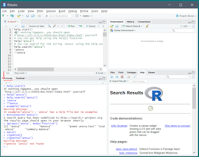
The function help.start() opens a browser window with access to introductory and advanced manuals, FAQs, and reference materials.
> help.start()R help functions :
| Function | Action |
| > help.start() | General help |
| > help("anova") or ?anova | Help on function "anova" (quotation marks optional) |
| > help.search("anov") or ??anov | Searches the help system for instances of the string "anov" |
| > example("anova") | Examples of function "anova" (quotation marks optional) |
| > RSiteSearch("anova") | Searches for the string foo in online help manuals and archived mailing lists |
| > apropos("anova", mode="function") | Lists all available functions with "anova" in their name |
| > data() | Lists
all available example datasets contained in currently loaded packages |
| > vignette() | Lists all available vignettes(documentation) for currently installed packages |
| > vignette("anova") | Displays specific vignettes(documentation) for topic "anova" |
The Workspace :
The workspace is your current R working environment and includes any user-defined objects (vectors, matrices, functions, data frames, and lists).
The current working directory is the directory from which R will read files and to which it will save results by default. You can find out what the current working directory is by using the getwd() function. You can set the current working directory by using the setwd() function.
Functions for managing the R workspace:
| Function | Action |
| > getwd() | Lists the current working directory. |
| > setwd("mydirectory") | Changes the current working directory to mydirectory |
| > ls() | Lists the objects in the current workspace. |
| > rm(objectlist) | Removes (deletes) one or more objects. |
| > help(options) | Provides information about available options. |
| > options() | Lets you view or set current options. |
| > history(#) | Displays your last # commands (default = 25). |
| > savehistory("myfile") | Saves the commands history to myfile (default =.Rhistory). |
| > loadhistory("myfile") | Reloads a command’s history (default = .Rhistory). |
| > save.image("myfile") | Saves the workspace to myfile (default = .RData). |
| > save(objectlist, file="myfile") | Saves specific objects to a file. |
| > load("myfile") | Loads a workspace into the current session. |
| > q() | Quits R. You’ll be prompted to save the workspace. |
Packages :
to the analysis of psychological tests.
Packages are collections of R functions, data, and compiled code in a well-defined format.
The directory where packages are stored on your computer is called the library.
The function .libPaths() shows you where your library is located, and the function library() shows you what packages you’ve saved in your library.
R comes with a standard set of packages (including base, datasets, utils, grDevices, graphics, stats, and methods). They provide a wide range of functions and datasets that are available by default. Other packages are available for download and installation.
Once installed, they must be loaded into the session in order to be used. The command search() tells you which packages are loaded and ready to use.
Installing a Package :
A number of R functions let you manipulate packages. To install a package for the first time, use the install.packages() command. For example, install.packages() without options brings up a list of CRAN mirror sites. Once you select a site, you’re presented with a list of all available packages. Selecting one downloads and installs it.
If you know what package you want to install, you can do so directly by providing it as
an argument to the function.
For example, the gclus package contains functions for creating enhanced scatter plots. You can download and install the package with the command install.packages("gclus").
You only need to install a package once. But like any software, packages are often updated by their authors. Use the command update.packages() to update any packages that you’ve installed. To see details on your packages, you can use the installed.packages() command. It lists the packages.
You only need to install a package once. But like any software, packages are often updated by their authors. Use the command update.packages() to update any packages that you’ve installed. To see details on your packages, you can use the installed.packages() command. It lists the packages.
Loading a package :
Installing a package downloads it from a CRAN mirror site and places it in your library.
To use it in an R session, you need to load the package using the library() command.
For example, to use the package gclus, issue the command library(gclus).Of course, you must have installed a package before you can load it.
You’ll only have to load the package once in a given session. If desired, you can customize your startup environment to automatically load the packages you use most often.
Learning about a Package :
When you load a package, a new set of functions and datasets becomes available.Small illustrative datasets are provided along with sample code, allowing you to try out the new functionalities.
When you load a package, a new set of functions and datasets becomes available.Small illustrative datasets are provided along with sample code, allowing you to try out the new functionalities.
The help system contains a description of each function(along with examples) and information about each dataset included. Entering help(package="package_name") provides a brief description of the package and an index of the functions and datasets included. Using help() with any of these function or dataset names provides further details. The same information can be downloaded as a PDF manual from CRAN.
R Operators :
R has several operators to perform tasks including arithmetic, logical and bitwise operations
R has several operators to perform tasks including arithmetic, logical and bitwise operations
R Arithmetic Operators :
The Arithmetic operators are used to carry out mathematical operations like addition and multiplication. Here is a list of arithmetic operators available in R.
| Operator | Description |
| + | Addition |
| - | Subtraction |
| * | Multiplication |
| / | Division |
| ^ | Exponent |
| %% | Modulus (Remainder from division) |
| %/% | Integer Division |
Example:
#Assigning the values to variables
> x <- 4
> y <- 15
#Performing some athematic operations
> x+y
#result
[1] 19
> x-y
[1] -11
> x*y
[1] 60
> y/x
[1] 3.75
> y%/%x
[1] 3
> y%%x
[1] 3
> y^x
#result
[1] 50265
R Relational Operators :
Relational operators are used to compare between values. Here is a list of relational operators available in R.
Example:
#Assigning the values to variables
> x <- 4
> x <- 4
> y <- 15
#Performing some athematic operations
> x+y
#result
[1] 19
> x-y
[1] -11
> x*y
[1] 60
> y/x
[1] 3.75
> y%/%x
[1] 3
> y%%x
[1] 3
> y^x
#result
[1] 50265
R Relational Operators :
Relational operators are used to compare between values. Here is a list of relational operators available in R.
| Operator | Description |
| < | Less than |
| > | Greater than |
| <= | Less than or equal to |
| >= | Greater than or equal to |
| == | Equal to |
| != | Not equal to |
Example:
#Assigning the values to variables
> x <- 4
> y <- 15
#Performing some relational operations
> x<y
#result
[1] TRUE
#Performing some relational operations
> x<y
#result
[1] TRUE
> x>y
[1] FALSE
> x<=5
[1] TRUE
> y>=20
[1] FALSE
> y == 16
[1] TRUE
> x != 5
#result
[1] FALSE
> x<=5
[1] TRUE
> y>=20
[1] FALSE
> y == 16
[1] TRUE
> x != 5
#result
[1] FALSE
R Logical Operators :
R Logical Operators :
Logical operators are used to carry out Boolean operations like AND, OR etc.
| Operator | Description |
| ! | Logical NOT |
| & | Element-wise logical AND |
| && | Logical AND |
| | | Element-wise logical OR |
| || | Logical OR |
Operators & and | perform element-wise operation producing result having length of the longer operand.
But && and || examines only the first element(the Scalar vectors) of the operands resulting into a single length logical vector.
Zero is considered FALSE and non-zero numbers are taken as TRUE.
Example:
#Assigning the values to variables
#c will concatenate the elements inside it.
#Performing some logical operations
> !x
#result
[1] FALSE TRUE TRUE FALSE
> x&y
#result
[1] FALSE FALSE FALSE TRUE
> x&&y
#result
[1] FALSE
> x[1] && y[1]
[1] False
> x|y
#result
[1] TRUE TRUE FALSE TRUE
> x||y
#result
[1] TRUE
R Assignment Operators:
These operators are used to assign values to variables.
The operators <- Leftwards assignment is used to assign to variable in the same environment.
The <<- operator is used for assigning to variables in the parent environments (more like global assignments). The rightward assignments, although available are rarely used.
> x <- 5
> x[1] 5
> 10 -> x
> x[1] 10
R Data Types :
In general while doing programming in any programming language, you need to use various variables to store various information. Variables are nothing but reserved memory locations to store values. This means that, when you create a variable you reserve some space in the memory.
You may like to store information of various data types like character, wide character,integer, floating point, double floating point, Boolean etc. Based on the data type of a variable, the operating system allocates memory and decides what can be stored in the reserved memory.
Unlike in many programming languages like C and java in R, the variables are not required to declared as some data type., you don’t have to declare an object’s data type or allocate space for it. The type is determined implicitly from the object’s contents, and the size grows or shrinks automatically depending on the type and number of elements the object contains.
The following are most widely used Data Type Objects in R.
Vectors
Lists
Matrices
Arrays
Factors
Data Frames
We will discuss in detail about each Object in upcoming tutorials; for now we will discuss about the basic data types of Vectors here..
Vectors :
There are two fundamental data types: Atomic Vectors and Generic Vectors
Atomic vectors are arrays that contain a single data type.
Generic vectors, also called Lists, are collections of atomic vectors.
A matrix is an atomic vector that has a dimension attribute, dim, containing two elements
(number of rows and number of columns).
An array is an atomic vector with a dim attribute that has three or more elements.
Factors are nominal or ordinal variables. They’re stored and treated specially in R.
Data frames are a special type of list, where each atomic vector in the collection has the same length.
The elements of a vector must all have the same mode, or data type. You can have a vector consisting of three character strings (of mode character) or three integer elements (of mode integer), but not a vector with one integer element and two character string elements.
Scalars, the individual numbers are actually one-element vectors.
> x <- 8
> x
[1] 8
[1] here signifies that the following row of numbers begins with element 1 of a vector—in this case, x[1]. So you can see that R was indeed treating x as a vector, albeit a vector with just one element.
Below are the basic data types of the atomic vectors, also termed as the classes of vectors. The other R-Objects are built upon the atomic vectors.
A) Numeric
Decimal values are called numerics in R. It is the default computational data type. If we assign a decimal value to a variable x as follows, x will be of numeric type.
> x <- 10.5 # assign a decimal value
> x # print the value of x
[1] 10.5
> class(x) # print the class name of x
[1] "numeric"
Furthermore, even if we assign an integer to a variable k, it is still being saved as a numeric value.
> k <-1
> k # print the value of k
[1] 1
> class(k) # print the class name of k
[1] "numeric"
The fact that k is not an integer can be confirmed with the is.integer function.
> is.integer(k) # is k an integer?
[1] FALSE
B) Integer:
In order to create an integer variable in R, we invoke the as.integer function. We can be assured that y is indeed an integer by applying the is.integer function.
> y = as.integer(3)
> y # print the value of y
[1] 3
> class(y) # print the class name of y
[1] "integer"
> is.integer(y) # is y an integer?
[1] TRUE
Incidentally, we can coerce a numeric value into an integer with the same as.integer function.
> as.integer(3.14) # coerce a numeric value
[1] 3
And we can parse a string for decimal values in much the same way.
> as.integer("5.27") # coerce a decimal string
[1] 5
On the other hand, it is erroneous trying to parse a non-decimal string.
> as.integer("Joe") # coerce an non−decimal string
[1] NA Warning message:
NAs introduced by coercion
Zero is considered FALSE and non-zero numbers are taken as TRUE.
Example:
#Assigning the values to variables
#c will concatenate the elements inside it.
> x <- c(TRUE,FALSE,0,6)
> y <- c(FALSE,TRUE,FALSE,TRUE)#Performing some logical operations
> !x
#result
[1] FALSE TRUE TRUE FALSE
> x&y
#result
[1] FALSE FALSE FALSE TRUE
> x&&y
#result
[1] FALSE
> x[1] && y[1]
[1] False
> x|y
#result
[1] TRUE TRUE FALSE TRUE
> x||y
#result
[1] TRUE
R Assignment Operators:
These operators are used to assign values to variables.
| Operator | Description |
| <-, <<- | Leftwards assignment |
| ->, ->> | Rightwards assignment |
The operators <- Leftwards assignment is used to assign to variable in the same environment.
The <<- operator is used for assigning to variables in the parent environments (more like global assignments). The rightward assignments, although available are rarely used.
> x <- 5
> x[1] 5
> 10 -> x
> x[1] 10
R Data Types :
In general while doing programming in any programming language, you need to use various variables to store various information. Variables are nothing but reserved memory locations to store values. This means that, when you create a variable you reserve some space in the memory.
You may like to store information of various data types like character, wide character,integer, floating point, double floating point, Boolean etc. Based on the data type of a variable, the operating system allocates memory and decides what can be stored in the reserved memory.
Unlike in many programming languages like C and java in R, the variables are not required to declared as some data type., you don’t have to declare an object’s data type or allocate space for it. The type is determined implicitly from the object’s contents, and the size grows or shrinks automatically depending on the type and number of elements the object contains.
The following are most widely used Data Type Objects in R.
Vectors
Lists
Matrices
Arrays
Factors
Data Frames
We will discuss in detail about each Object in upcoming tutorials; for now we will discuss about the basic data types of Vectors here..
Vectors :
There are two fundamental data types: Atomic Vectors and Generic Vectors
Atomic vectors are arrays that contain a single data type.
Generic vectors, also called Lists, are collections of atomic vectors.
A matrix is an atomic vector that has a dimension attribute, dim, containing two elements
(number of rows and number of columns).
An array is an atomic vector with a dim attribute that has three or more elements.
Factors are nominal or ordinal variables. They’re stored and treated specially in R.
Data frames are a special type of list, where each atomic vector in the collection has the same length.
The elements of a vector must all have the same mode, or data type. You can have a vector consisting of three character strings (of mode character) or three integer elements (of mode integer), but not a vector with one integer element and two character string elements.
Scalars, the individual numbers are actually one-element vectors.
> x <- 8
> x
[1] 8
[1] here signifies that the following row of numbers begins with element 1 of a vector—in this case, x[1]. So you can see that R was indeed treating x as a vector, albeit a vector with just one element.
Below are the basic data types of the atomic vectors, also termed as the classes of vectors. The other R-Objects are built upon the atomic vectors.
A) Numeric
Decimal values are called numerics in R. It is the default computational data type. If we assign a decimal value to a variable x as follows, x will be of numeric type.
> x <- 10.5 # assign a decimal value
> x # print the value of x
[1] 10.5
> class(x) # print the class name of x
[1] "numeric"
Furthermore, even if we assign an integer to a variable k, it is still being saved as a numeric value.
> k <-1
> k # print the value of k
[1] 1
> class(k) # print the class name of k
[1] "numeric"
The fact that k is not an integer can be confirmed with the is.integer function.
> is.integer(k) # is k an integer?
[1] FALSE
B) Integer:
In order to create an integer variable in R, we invoke the as.integer function. We can be assured that y is indeed an integer by applying the is.integer function.
> y = as.integer(3)
> y # print the value of y
[1] 3
> class(y) # print the class name of y
[1] "integer"
> is.integer(y) # is y an integer?
[1] TRUE
Incidentally, we can coerce a numeric value into an integer with the same as.integer function.
> as.integer(3.14) # coerce a numeric value
[1] 3
And we can parse a string for decimal values in much the same way.
> as.integer("5.27") # coerce a decimal string
[1] 5
On the other hand, it is erroneous trying to parse a non-decimal string.
> as.integer("Joe") # coerce an non−decimal string
[1] NA Warning message:
NAs introduced by coercion
Often, it is useful to perform arithmetic on logical values. Like the C language, TRUE has the value 1, while FALSE has value 0. > as.integer(TRUE) # the numeric value of TRUE
[1] 1
> as.integer(FALSE) # the numeric value of FALSE
[1] 0
[1] 1
> as.integer(FALSE) # the numeric value of FALSE
[1] 0
C) Complex:
A complex value in R is defined via the pure imaginary value i.
> z <- 1 + 2i # create a complex number
> z # print the value of z
[1] 1+2i
> class(z) # print the class name of z [1] "complex"
> z <- 1 + 2i # create a complex number
> z # print the value of z
[1] 1+2i
> class(z) # print the class name of z [1] "complex"
The following gives an error as −1 is not a complex value.
> sqrt(−1) # square root of −1
[1] NaN
Warning message:
In sqrt(−1) : NaNs produced
Instead, we have to use the complex value −1 + 0i.
> sqrt(−1+0i) # square root of −1+0i
[1] 0+1i
An alternative is to coerce −1 into a complex value.
> sqrt(as.complex(−1))
[1] 0+1i
A logical value is often created via comparison between variables.
> x <- 4; y <- 7 # sample values
> z = x > y # is x larger than y?
> z # print the logical value
[1] FALSE
> class(z) # print the class name of z
[1] "logical"
Standard logical operations are "&" (and), "|" (or), and "!" (negation).
> u <- TRUE; v <- FALSE
> u & v # u AND v
[1] FALSE
> u | v # u OR v
[1] TRUE
> !u # negation of u
[1] FALSE
Further details and related logical operations can be found in the R documentation.
> help("&")
E) Character :
A character object is used to represent string values in R. We convert objects into character values with the as.character() function:
> x <- as.character(3.14)
> x # print the character string
[1] "3.14"
> class(x) # print the class name of x
[1] "character"
> x <- as.character(3.14)
> x # print the character string
[1] "3.14"
> class(x) # print the class name of x
[1] "character"
Two character values can be concatenated with the paste function.
> fname <- "James"; lname <-"Bond"
> paste(fname, lname)
[1] "James Bond"
However, it is often more convenient to create a readable string with the sprintf function, which has a C language syntax.
> sprintf("%s has %d dollars", "Ram", 100)
[1] "Ram has 100 dollars"
> sprintf("%s has %d dollars", "Ram", 100)
[1] "Ram has 100 dollars"
To extract a substring, we apply the substr function. Here is an example showing how to extract the substring between the third and twelfth positions in a string.
> substr("Mary has a little lamb.", start=3, stop=12)
[1] "ry has a l"
And to replace the first occurrence of the word "little" by another word "big" in the string, we apply the sub function.
> sub("little", "big", "Mary has a little lamb.")
[1] "Mary has a big lamb."
More functions for string manipulation can be found in the R documentation.
> help("sub")
We will discuss about each below Object in detail in upcoming tutorials.
Vectors
Lists
Matrices
Arrays
Factors
Data Frames
Lists
Matrices
Arrays
Factors
Data Frames
--------------------------------------------------------------------------------------------------------
Thanks, TAMATAM ; Business Intelligence & Analytics Professional
Thanks, TAMATAM ; Business Intelligence & Analytics Professional
--------------------------------------------------------------------------------------------------------


No comments:
Post a Comment
Hi User, Thank You for visiting My Blog. If you wish, please share your genuine Feedback or comments only related to this Blog Posts. It is my humble request that, please do not post any Spam comments or Advertising kind of comments, which will be Ignored.