How to use dplyr() Package for Data Wrangling in R Programming

Data Wrangling with functions of dplyr() Package in R
The package "dplyr" provides easy tools for the most common data manipulation tasks. It is built to work directly with data frames, with many common tasks optimized by being written in a compiled language (C++).
An additional feature is the ability to work directly with data stored in an external database. The benefits of doing this are that the data can be managed natively in a relational database, queries can be conducted on that database, and only the results of the query are returned.
The "dplyr" package is a grammar of data manipulation, providing a consistent set of verbs that help you solve the most common data manipulation challenges.
The "dplyr" package addresses a common problem with R is that, all operations are conducted in-memory and thus the amount of data you can work with is limited by available memory.
The database connections feature of the "dplyr" package essentially remove that limitation in that you can connect to a database of many hundreds of GB, conduct queries on it directly, and pull back into R only what you need for analysis.
The "dplyr" package belongs to the family of "tidyverse" packages (ggplot2, dplyr, tidyr, readr, purr, tibble,hms, stringr, lubridate, forcats, DBI, haven, httr, jsonlite, readxl, rvest, xml2, modelr, broom)

The "dplyr" is a package for data manipulation, written and maintained by Hadley Wickham. It provides some great, easy-to-use functions that are very handy when performing exploratory data analysis and manipulation

You can learn more about this package using vignette("dplyr")

The following are the standard functions available in dplyr package :

select(): Select the variables from a dataset
filter():  Apply the fitters on the variables of a dataset
mutate(): Create the new variables by using information from existing variables
group_by() and summarize(): Create summary statistics on grouped data
arrange(): Sort/ordering the results
count(): Count discrete values

>install.packages("dplyr")

>library("dplyr")

Scenario :

Now we will read and explore the dataset then we perform various functions on the dataset.

> dt_sales<-read.csv(fpath,header=T,sep="\t",dec=",",as.is=T,na.strings = c("NULL","NA","na",""))

#Formatting columns :

We will format few of the columns of the above dataset

> dt_sales$Order_Date<-as.Date(dt_sales$Order_Date,"%m/%d/%Y")
> dt_sales$FiscalQuarter<-as.factor(dt_sales$FiscalQuarter)
> dt_sales$Region_Name<-as.factor(dt_sales$Region_Name)
> dt_sales$Cust_Segment<-as.factor(dt_sales$Cust_Segment)

Exploring dataset :

Now we will explore the dataset using various functions

> str(dt_sales)

> summary(dt_sales)

> tbl_df(dt_sales)

OR

> print(tbl_df(dt_sales),n=10)

> glimpse(dt_sales)

Functions of dplyr package :

1. select() :

The selection function is used to select the Variables from a dataset. The first argument to this function is the data frame (surveys), and the subsequent arguments are the columns to keep.
As well as using existing functions like : and c(), there are a number of special functions that work inside select () :starts_with(), ends_with(), contains() , matches(), num_range(), one_of(), everything()
To drop variables from select() we use - prefix to columns.# Selecting the entire dataset :

>select(dt_sales,everything())

> tbl_df(select(dt_sales,everything())) 

Note : every where I used tbl_df () to limit/fit the results on the screen.

#Selecting only specific Variables( by passing Variables Name or Number)

> tbl_df(select(dt_sales,Order_Id,FiscalQuarter,Gross_Sales))
OR
> tbl_df(select(dt_sales,c(1,3,9)))

#Selecting sequence of Variables
> tbl_df(select(dt_sales,Order_Id:Cust_Segment))
OR

> tbl_df(select(dt_sales,1:5))

#Removing specific/sequence of Variables from selection

We can remove the specific/sequence of Variables from selection by specifying their Name(s) or Number(s)

>tbl_df(select(dt_sales,-Order_Date,-FiscalQuarter,-Region_Name,-Cust_Segment))
OR
> tbl_df(select(dt_sales,-2,-3,-4,-5))
OR
> tbl_df(select(dt_sales,-(Order_Date:Cust_Segment)))
OR
> tbl_df(select(dt_sales,-(2:5))

#Exclude in between Variables from selection

>tbl_df(select(dt_sales,(1:9),-2,-5,-8))

Utility functions of select() :

Utility functions existing in select(), summarise_each() and mutate_each() in dplyr as well as some functions in the tidyr package.
Seven functions existed in the utility functions of select().
a) starts_with(match, ignore.case = TRUE)
b) ends_with(match, ignore.case = TRUE)
c) contains(match, ignore.case = TRUE)
d) matches(match, ignore.case = TRUE)
e) num_range(prefix, range, width = NULL)
f) one_of(...)
g) everything()
#Selecting the Variables based on whose names starts with a specified string

> tbl_df(select(dt_sales,starts_with("Order",ignore.case=T)))

#Selecting the Variables based on whose names ends with a specified string

> tbl_df(select(dt_sales,ends_with("e",ignore.case=T)))

#Selecting the Variables whose names contains a specified string

> tbl_df(select(dt_sales,contains("eg",ignore.case=T)))

#Selecting the Variables whose names pattern matches(partial/full) to a specified string

The matches() picks Variables based on a regular expression matching string.

> tbl_df(select(dt_sales,matches("eg",ignore.case=T)))

#Selecting the Variables based on number range in their Names

When the numbers were included in column names, num_range() function will be useful.
In this example, we will change the column names with prefix "Var" to be like Var1–Var9 and execute num_range() command for the data set.

> dt2_sales<-dt_sales
> colnames(dt2_sales) <- sprintf("Var%d", 1:9)

By specifying as num_range("Var",1:5), columns Var1 to Var5 can be identified.

 >tbl_df(select(dt2_sales,num_range("Var",1:5)))

Numbers in the column names are not necessarily sequential, we can specify them individually as num_range("Var", c(2, 15))
> tbl_df(select(dt2_sales,num_range("Var",c(1,3,4,9))))

When column names were padded, the column name was shown as Var01.Here, the argument width in num_range() will be useful. We now try this process for a data that changes the column names as Var01–Var09.
>colnames(dt2_sales) <- sprintf("Var%02d", 1:9)

>tbl_df(select(dt2_sales,num_range("Var",1:5,width=2)))

#Selecting the one of the Variables of specified Vector

When a column is named as a vector or character string, one_of() might be useful.

> V_VarNames<-c("Order_Id","Quarter","Cust_Segment","Region","Gross_Sales")

Here, again I am using the original dataset "dt_sales"
> tbl_df(select(dt_sales,one_of(V_VarNames)))

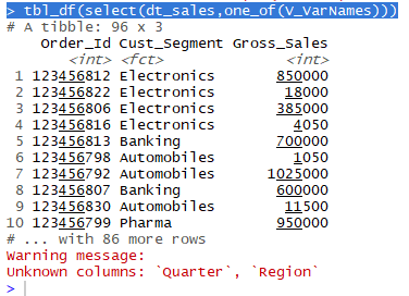
Note:

A Warning message will be thrown for Unknown Columns specified in the Vector.

2. filter() :
The filter() function is used to filter the observations based on specific criteria passed as a filter on Variables.
# Applying filter on specific variables ; Output all Variables

> filter(dt_sales, Region_Name %in% c("Europe","Asia"),Order_Date<="2014-05-30")

OR
> filter(dt_sales, Region_Name %in% c("Europe","Asia") & Order_Date<="2014-05-30")

# Applying filter on specific variables ; Output only selected Variables

> select(filter(dt_sales, Region_Name %in% c("Europe","Asia"),Order_Date<="2014-05-30"), c(1,3:5,9))
OR
>select(filter(dt_sales, Region_Name %in% c("Europe","Asia") & Order_Date<="2014-05-30"), c(1,3:5,9))
OR
We can write about code using the Pipe/Chain operator "%>%". The Pipes let you take the output of one function and send/connect it directly to the next, which is useful when you need to do many things to the same dataset. Pipes in R look like %>% and are made available via the magrittr package, installed automatically with dplyr.
> dt_sales %>%

filter(Region_Name %in% c("Europe","Asia") & Order_Date<="2014-05-30") %>%
select(1,3:5,9)

> select(filter(dt_sales, Region_Name %in% c("Europe","Asia")& Order_Date<="2014-05-30", Gross_Sales<=20000),c(1,3:5,9))

3. mutate () :

The mutate() function is used create new Variables based on the values of existing Variables.

# Creating new calculated Variables(Disc, Net_Sales) ; Output all variables

>tbl_df(mutate(dt_sales,Disc.=(0.02*Gross_Sales),Net_Sales=(Gross_Sales-COGS)))

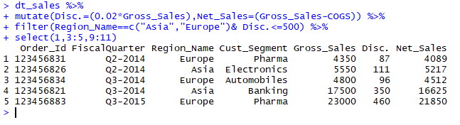
# Creating new Variable(Disc) ; include new Variable in Filter then Select specific Variables

>dt_sales %>%
mutate(Disc.=(0.02*Gross_Sales),Net_Sales=(Gross_Sales-COGS)) %>%
filter(Region_Name %in% c("Asia","Europe") & Disc.<=500) %>%
select(1,3:5,9:11)

4. summarize () / summarise () :
The summarise() function is used to summarise multiple values into a single value.

The group_by() is often used together with summarize() or summarise() function, which collapses each group into a single-row summary of that group.
The group_by() takes the categorical variables as arguments for which you want to calculate the summary statistics (eg: Mean).
The group_by function is used to group data by one or more variables.. ungroup() removes grouping.
#Grouping the data by specific variables

> group_by(dt_sales,FiscalQuarter,add=FALSE)

Note :
When add = FALSE, the default, group_by() will override existing groups on the dataset. To add to the existing groups, use add = TRUE
#Summarizing the data by grouping specific variables
>summarize(group_by(dt_sales,FiscalQuarter,add=FALSE), Avg_Sales=mean(Gross_Sales, na.rm = T))

5. arrange() :
The arrange function is used to sort the data ascending/descending by specified variables.
# Arrange data by Sorting Asc by Region_Name and Desc by Gross_Sales variables
>arrange(dt_sales,Region_Name , desc(Gross_Sales))
>head(arrange(dt_sales,Region_Name , desc(Gross_Sales)),n=30)
# Arrange the Grouped data(by FiscalQuarter) , Sort by Gross_Sales Desc; Leave the previous grouping order as it is.
> dt_sales %>%
  group_by(FiscalQuarter,add=FALSE) %>%
  arrange(desc(Gross_Sales),.by_group=TRUE)
Note :
In arrange() function If .by_group=TRUE, it will sort first by grouping variables the Sort applies by specified variable to grouped data.

6. count() :
The count function counts the no.of observations per group. It is slightly similar to the table function in the base package.

#Count of observations group by FiscalQuarter variable
> count(dt_sales,FiscalQuarter)

#Count of observations group by Cust_Segment variable
> count(dt_sales,Cust_Segment)

--------------------------------------------------------------------------------------------------------
Thanks, TAMATAM ; Business Intelligence & Analytics Professional
--------------------------------------------------------------------------------------------------------