Analyze and Impute the Missing Data with VIM and Mice Packages in R Programming
In the field of data science, while doing data analysis, we may come across missing values which can potentially impact our analysis and data model. Handling missing values is one of crucial thing for further analysis of data. The reason for missing data is often not collected or incompletely collected.
Types of Missing Data :
A) Missing Completely At Random (MCAR) :
B) Missing At Random (MAR):
MAR, means there is a systematic relationship between the probability of missing values and the observed data, but not the missing data.
C) Missing Not At Random (MNAR):
When observations are neither MCAR nor MAR, are classified as Missing Not At Random (MNAR), i.e. the probability of an observation being missing depends on the unobserved measurements. In this scenario, the value of the unobserved responses not depends on the values observed previously on the analysis variable, and thus, future observations cannot be predicted without bias by the model.
Missing not at random data is a more serious issue and in that case we have to review the data gathering process further and try to understand why the information is missing.
For instance, if most of the people in a survey did not answer a certain question, why did they do that? Was the question unclear?.
Example :
Suppose you are modelling Weight (Y) as a function of Gender(X). Some people wouldn't disclose their Weight, so you are missing some values for Y.
There are three possible mechanisms for the nondisclosure:
There may be no particular reason why some respondents told you their weights and others didn't. That is, the probability that Y is missing may has no relationship to X or Y. In such a case our data is Missing Completely At Random (MCAR).
One Gender group may be less likely to disclose its weight. That is, the probability that Y is missing depends only on the value of X. Such data are Missing At Random (MAR).
Fat or Lean people may be less likely to disclose their weight. That is, the probability that Y is missing depends on unobserved values of Y itself. Such data are not missing at random but Missing Not At Random (MNAR).By handling missing values effectively we can reduce bias and can produce powerful models.
If the dataset is very large and the number of missing values in the data are very small (typically less than 5% as the case may be), the values can be ignored and analysis can be performed on the rest of the data.
Sometimes, the number of missing values are too large then we have to ‘impute' the missing values instead of dropping them from the data.
If the Missing values for a Variable is greater than 20-25 %, then we have to gather more data on that Variable or we can drop it from the Data Model.
In R, the following are the popular packages available for imputing missing values:
MICE
Amelia
missForest
Hmisc
mi
Checking Percentage of Missing Observations in Dataset:


 Apparently, only the Ozone variable is statistically significant.
In the field of data science, while doing data analysis, we may come across missing values which can potentially impact our analysis and data model. Handling missing values is one of crucial thing for further analysis of data. The reason for missing data is often not collected or incompletely collected.
Types of Missing Data :
A) Missing Completely At Random (MCAR) :
Missing Completely at Random, MCAR, means there is no relationship between the missingness of the data and the observed or missing values. MCAR occurs when there is a simple probability that data will be missing, and that probability is unrelated to anything else in your study. Those missing data points are a random subset of the data. There is nothing systematic going on that makes some data more likely to be missing than others.
For the dependent variable, if the probability of an observation being missing does not depend on observed or unobserved measurements then the observation is Missing Completely At Random (MCAR).
For example, In a Lab, some Researchers may have missing laboratory values because a batch of lab samples process was failed due to processing machine fault. In these instances, the missing data reduce the analyzable population of the study and consequently, the statistical power, but do not introduce bias. When data are MCAR, the data which remain can be considered a simple random sample of the full data set of interest. MCAR is generally regarded as a strong and often unrealistic assumption.
B) Missing At Random (MAR):
If the probability of an observation being missing depends only on observed measurements then the observation is Missing At Random (MAR).
For example, a Psychiatrist conducting a depression survey data that may encounter MAR, if Male participants are less likely to complete a survey about depression severity than the Female participants. That is, if probability of completion of the survey is related to their Gender(which is fully observed) but not the severity of their depression, then the data may be regarded as MAR.
For example, a Psychiatrist conducting a depression survey data that may encounter MAR, if Male participants are less likely to complete a survey about depression severity than the Female participants. That is, if probability of completion of the survey is related to their Gender(which is fully observed) but not the severity of their depression, then the data may be regarded as MAR.
C) Missing Not At Random (MNAR):
Missing not at random data is a more serious issue and in that case we have to review the data gathering process further and try to understand why the information is missing.
For instance, if most of the people in a survey did not answer a certain question, why did they do that? Was the question unclear?.
Example :
Suppose you are modelling Weight (Y) as a function of Gender(X). Some people wouldn't disclose their Weight, so you are missing some values for Y.
There are three possible mechanisms for the nondisclosure:
There may be no particular reason why some respondents told you their weights and others didn't. That is, the probability that Y is missing may has no relationship to X or Y. In such a case our data is Missing Completely At Random (MCAR).
One Gender group may be less likely to disclose its weight. That is, the probability that Y is missing depends only on the value of X. Such data are Missing At Random (MAR).
Fat or Lean people may be less likely to disclose their weight. That is, the probability that Y is missing depends on unobserved values of Y itself. Such data are not missing at random but Missing Not At Random (MNAR).By handling missing values effectively we can reduce bias and can produce powerful models.
If the dataset is very large and the number of missing values in the data are very small (typically less than 5% as the case may be), the values can be ignored and analysis can be performed on the rest of the data.
Sometimes, the number of missing values are too large then we have to ‘impute' the missing values instead of dropping them from the data.
If the Missing values for a Variable is greater than 20-25 %, then we have to gather more data on that Variable or we can drop it from the Data Model.
Data without missing values can be summarized by some statistical measures such as Mean and Variance. Hence, we always have to fill or ‘impute’ missing values in such a way that some of these measures do not change.For numerical data, one can impute with the "Mean" of the data so that the overall mean does not change. In this process, however, the Variance decreases and changes.
In some cases such as in time series, one can take the Moving average of a window and replaces missing values with the mean of all existing values in that window. This method is also known as Method of moving averages.
In some cases such as in time series, one can take the Moving average of a window and replaces missing values with the mean of all existing values in that window. This method is also known as Method of moving averages.
For non-numerical data, ‘imputing’ with "Mode" is a common choice.
Important Note :
Please note that first we need to remove the outliers from the dataset, then we have to do the Missing values Treatment, and finally we have to fit that to a Data model. The outliers treatment is not covered in this article. We assume that there was no outliers in the dataset.
Important Note :
Please note that first we need to remove the outliers from the dataset, then we have to do the Missing values Treatment, and finally we have to fit that to a Data model. The outliers treatment is not covered in this article. We assume that there was no outliers in the dataset.
In R, the following are the popular packages available for imputing missing values:
MICE
Amelia
missForest
Hmisc
mi
The MICE(Multivariate Imputations via Chained Equations) package is one of the fastest and probably a gold standard for imputing values.
MICE Package :
MICE (Multivariate Imputation via Chained Equations) is one of the commonly used package by R users. Creating multiple imputations as compared to a single imputation (such as Mean) takes care of uncertainty in missing values.
MICE assumes that the missing data are Missing at Random (MAR), which means that the probability that a value is missing depends only on observed value and can be predicted using them. It imputes data on a variable by variable basis by specifying an imputation model per variable.
Precisely, the methods used by the MICE Package are:
PMM (Predictive Mean Matching) - For Numeric variables
logreg(Logistic Regression) - For Factor/Categorical/Binary Variables ( with 2 levels)
polyreg (Bayesian polytomous regression) - For Factor/Categorical Variables (>= 2 levels)
Proportional odds model - For Factor/Categorical Variables (ordered, >= 2 levels)
VIM (Visualization and Imputation of Missing Values ) Package :
> install.packages("VIM")
> install.packages("mice")
> library(VIM)
> library(mice)
In this post we are going to impute missing values using a the airquality dataset (available in R). Lets have a look at the original dataset.
> tbl_df(airquality)
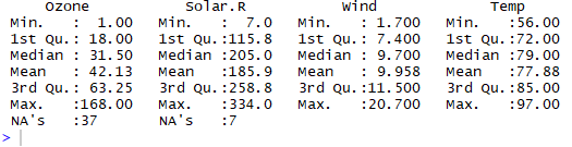
 > summary(airquality)
 For the purpose of Analysis I am reading this data set to another df "mydata" then remove some data points, and setting the NA's for the variables 3 and 4 in the dataset.
> mydata <- airquality
> mydata[4:10,3] <- rep(NA,7)
> mydata[1:5,4] <- NA
Also, We are removing the variables Month and Day from this Dataset as we are not using them in analysis.
> mydata <- mydata[-c(5,6)]
 We observed that Ozone is the variable with the most missing data points.
MICE Package :
MICE (Multivariate Imputation via Chained Equations) is one of the commonly used package by R users. Creating multiple imputations as compared to a single imputation (such as Mean) takes care of uncertainty in missing values.
MICE assumes that the missing data are Missing at Random (MAR), which means that the probability that a value is missing depends only on observed value and can be predicted using them. It imputes data on a variable by variable basis by specifying an imputation model per variable.
Example:
Suppose we have X1, X2….Xk variables. If X1 has missing values, then it will be regressed on other variables X2 to Xk. The missing values in X1 will be then replaced by predictive values obtained. Similarly, if X2 has missing values, then X1, X3 to Xk variables will be used in prediction model as independent variables. Later, missing values will be replaced with predicted values.
By default, linear regression is used to predict continuous missing values.
Logistic regression is used for categorical missing values.
Once this cycle is complete, multiple data sets are generated. These data sets differ only in imputed missing values. Generally, it’s considered to be a good practice to build models on these data sets separately and combining their results.
PMM (Predictive Mean Matching) - For Numeric variables
logreg(Logistic Regression) - For Factor/Categorical/Binary Variables ( with 2 levels)
polyreg (Bayesian polytomous regression) - For Factor/Categorical Variables (>= 2 levels)
Proportional odds model - For Factor/Categorical Variables (ordered, >= 2 levels)
VIM (Visualization and Imputation of Missing Values ) Package :
In R, the VIM Package is useful for visualization of missing and/or imputed values are introduced, which can be used for exploring the data and the structure of the missing and/or imputed values.
Depending on this structure of the missing values, the corresponding imputing methods may help to identify the mechanism for generating the values to impute for missing and allows to explore the data after imputing the missing values. In addition, the quality of imputation can be visually explored using various univariate, bivariate, multiple and multivariate plot methods.
Analyzing Missing Data Pattern with VIM and Mice Packages::
Now we will discuss about Analyzing the Missing Data with VIM Package and then Impute the Missing data with Mice Package in R.Analyzing Missing Data Pattern with VIM and Mice Packages::
> install.packages("VIM")
> install.packages("mice")
> library(VIM)
> library(mice)
In this post we are going to impute missing values using a the airquality dataset (available in R). Lets have a look at the original dataset.
> tbl_df(airquality)


> mydata <- airquality
> mydata[4:10,3] <- rep(NA,7)
> mydata[1:5,4] <- NA
Also, We are removing the variables Month and Day from this Dataset as we are not using them in analysis.
> mydata <- mydata[-c(5,6)]
> summary(mydata)

We Assume that the data is Missing At Random(MAR), too much missing data can be a problem too.
Usually a safe maximum threshold is 5% of the total for large datasets. If missing data for a certain Variable or Sample is more than 5% then you probably should leave that Variable or Sample out.
Checking Percentage of Missing Observations in Dataset:
Now we will check the Missing data by Variables(Columns) and Samples (Rows) and get to know where more than 5% of the data is Missing using a simple user defined function as follows..
> pMiss <- function(x)
{
sum(is.na(x))/length(x)*100
}
> apply(mydata,2,pMiss) # Percentage of Missing Observations by Variable
Ozone Solar.R Wind Temp
 We see that Ozone variable is missing almost 25% of the data points, therefore we might consider either dropping it from the analysis or gather more measurements for that variable.
> library(mice)
> md.pattern(mydata)
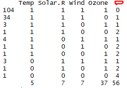

The above Output tells us that 104 samples are complete (no Missing values), 34 values are missed for the Ozone variable, 4 values are missed for the Solar.R variable and so on.
Now we will visualize and analyze the proportion of Missing data by variable using the VIM Package's aggregation plot.
Using the aggr() function helps to create an aggregated plot with the combination Histogram and a pattern chart.
> aggr_plot <- aggr(mydata, col=c('navyblue','red'), numbers=TRUE, sortVars=TRUE, labels=names(mydata), cex.axis=0.75, gap=3, ylab=c("Histogram of Missing Data", "Missing Data Pattern"))
Notes :

Variables sorted by number of missings:
Variable Count
24.183007 4.575163 4.575163 3.267974
> apply(data,1,pMiss) # Percentage of Missing Observations by Rows

The other variables are below the 5% threshold so we can keep them.
As far as the Samples are concerned, missing just one Variable leads to a 25% missing data per Sample. Samples that are missing 2 or more Variables (>50%), should be dropped from analysis if possible.
Using Mice for Analyzing the Missing data Pattern:
The Mice package provides a great function md.pattern() to get a better understanding of the pattern of Missing data.
>md.pattern(x, plot = TRUE)
The Mice package provides a great function md.pattern() to get a better understanding of the pattern of Missing data.
>md.pattern(x, plot = TRUE)
x - A data frame or a matrix containing the incomplete data. Missing values are coded as NA's.
plot - Should the missing data pattern be made into a pattern plot. Default is 'plot = TRUE'.
A summarized data from with ncol(x)+1 columns, in which each row corresponds to missing data pattern (1=observed, 0=missing). Rows and Columns are sorted in increasing amounts of missing information. The first column shows the count of observations, last column shows the count of variables with Missing data (respective Missing count in first column).
> md.pattern(mydata)

Now we will visualize and analyze the proportion of Missing data by variable using the VIM Package's aggregation plot.
Using the aggr() function helps to create an aggregated plot with the combination Histogram and a pattern chart.
> aggr_plot <- aggr(mydata, col=c('navyblue','red'), numbers=TRUE, sortVars=TRUE, labels=names(mydata), cex.axis=0.75, gap=3, ylab=c("Histogram of Missing Data", "Missing Data Pattern"))
Notes :
cex.axis - to specify the size of the x-axis text (Ozone, Solar.R, Wind..) and y-axis(0.00, 0.05 , 0.10...)
gap - to specify the width between the two plots.
Output:
gap - to specify the width between the two plots.
Output:

Variable Count
Ozone 0.24183007
Solar.R 0.04575163
Wind 0.04575163
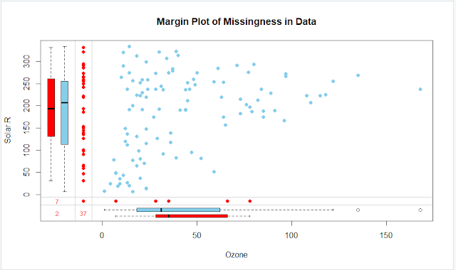
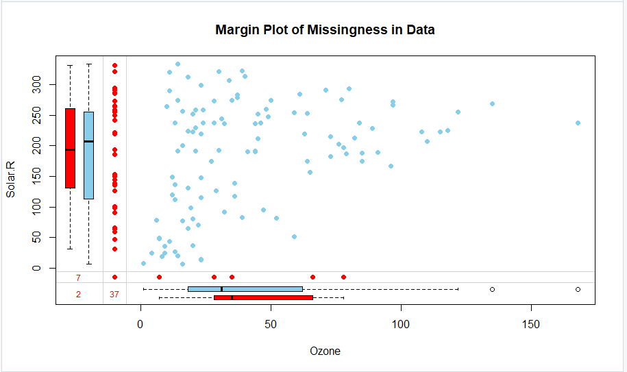
We can also visualize the data using the boxpot "marginplot" but using only two Variables at time to gain some interesting insights.
>marginplot(mydata[,c(1,2)],cex.numbers = 0.75,pch = 19,axes =T,col = c("skyblue", "red"),
xlab = "Ozone", ylab = "Solar.R",main="Margin Plot of Missingness in Data")
 Notes:
cex.numbers - argument to specify the size of the numbers( in left corner of plot 7,2, 37..)
pch - argument to specify the symbol of the dots on the plot.The red box plot on the left(y-axis) shows the distribution of values for the "Solar.R" variable with the missing values in "Ozone" variable, while the blue box plot shows the distribution of the remaining data points.
Solar.R 0.04575163
Wind 0.04575163
Temp 0.03267974
In the above charts, Histogram shows only the proportion(percentage) of Missing values. The Pattern chart shows the proportion of Non-Missing(Blue) and Missing(Red) values.
Now from this plot we understand that almost 70%(the total Blue proportions : 0.67+0.01..) of the observations are not missing any information in the data set, 22% of observations are missing the Ozone variable, and remaining ones shows missing patterns for other variables.We can also visualize the data using the boxpot "marginplot" but using only two Variables at time to gain some interesting insights.
>marginplot(mydata[,c(1,2)],cex.numbers = 0.75,pch = 19,axes =T,col = c("skyblue", "red"),
xlab = "Ozone", ylab = "Solar.R",main="Margin Plot of Missingness in Data")
cex.numbers - argument to specify the size of the numbers( in left corner of plot 7,2, 37..)
pch - argument to specify the symbol of the dots on the plot.The red box plot on the left(y-axis) shows the distribution of values for the "Solar.R" variable with the missing values in "Ozone" variable, while the blue box plot shows the distribution of the remaining data points.
Likewise for the Ozone (on x-axis) box plots at the bottom of the graph.
If our assumption of MAR data is correct, then we expect the red and blue box plots to be very similar.
If our assumption of MAR data is correct, then we expect the red and blue box plots to be very similar.
Imputing the missing data with Mice Package:
Now we will Impute the missing data with mice() function of mice package using Predictive Mean Method(PMM).
>impData <- mice(mydata,m=5,maxit=50,meth='pmm',seed=500)

 here, I have shown only few rows that imputed.

Mean value for Variable "Solar.R" before Imputation = 185.90
Mean value for Variable "Solar.R" after Imputation = 186
We noticed that there is not much variance in the Mean values of the Imputed variables before and after. It is looks like the Imputation process is good.
Inspecting the distribution of original and imputed data:
We can also Analyze & Inspect the distribution of original and Imputed data, using xyplot() and densityplot() functions.
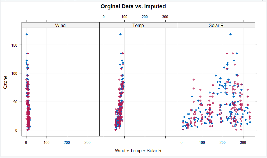
First of all we will use a scatterplot to plot Ozone against all the other variables
>library(lattice)
>xyplot(impData,Ozone ~ Wind+Temp+Solar.R, pch=18,cex=1.0, grid = TRUE,
main="Orginal Data vs. Imputed" )
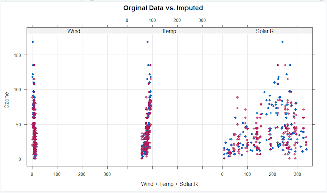 From the above plot we observed that the shape of the imputed values(in pink) matches to the shape of the observed(in blue) values. So that we can conclude that the imputed values are reasonable.
Now we will use a density plot to plot Ozone against all the other variables>impData <- mice(mydata,m=5,maxit=50,meth='pmm',seed=500)
>summary(impData)

Notes:
m=5 refers to the no.of imputed datasets should generate. Default value is 5.This means that we now have 5 imputed datasets. We can use either one of 5 as a final dataset.
maxit=50 refers to the max no.of iterations(you can specify the desired no) after that the dataset will created with imputed values.
meth='pmm' refers to the imputation method. In this case we are using predictive mean matching as imputation method. Other imputation methods also can be used, type methods(mice) for a list of the available imputation methods.
If you would like to check the imputed data for a variable say "Ozone", we can do it as below>impData$imp$Ozone

The output shows the imputed data for each observation (first column left) within each imputed dataset (first row at the top).
We can check the imputation method used for each variable as below
> impData$meth
Ozone Solar.R Wind Temp
> impData$meth
Ozone Solar.R Wind Temp
"pmm" "pmm" "pmm" "pmm"
Finally we can complete the imputation process using the complete() function.
> CompleteImpData <- complete(impData,1)
> CompleteImpData <- complete(impData,1)
The missing values have been replaced with the imputed values in the first dataset of the five datasets that were generated during the imputation process.
If you wish to use another dataset, just change the second parameter in the complete() function.
Now we will see the Summary statistics of the Imputed Dataset.
If you wish to use another dataset, just change the second parameter in the complete() function.
Now we will see the Summary statistics of the Imputed Dataset.
>summary(CompleteImpData)

Now we can compare the Summary of the Imputed Dataset with original Dataset to see is there any significant difference in the Mean values of each Variable.
>summary(airquality)

Goodness of fit of Imputation Process :
Finally we need to verify the Good of fit of the Imputed values, to check how good they are.
Simplest way is we compare the Mean values of Variables before Imputation and after the Imputation.
Mean value for Variable "Ozone" before Imputation = 42.13
Mean value for Variable "Ozone" after Imputation = 40.35Simplest way is we compare the Mean values of Variables before Imputation and after the Imputation.
Mean value for Variable "Ozone" before Imputation = 42.13
Mean value for Variable "Solar.R" before Imputation = 185.90
Mean value for Variable "Solar.R" after Imputation = 186
We noticed that there is not much variance in the Mean values of the Imputed variables before and after. It is looks like the Imputation process is good.
Inspecting the distribution of original and imputed data:
First of all we will use a scatterplot to plot Ozone against all the other variables
>library(lattice)
>xyplot(impData,Ozone ~ Wind+Temp+Solar.R, pch=18,cex=1.0, grid = TRUE,
main="Orginal Data vs. Imputed" )
>densityplot(impData, type="density",equal.widths =T ,main="Orginal Data vs. Imputed")

The density of the imputed data for each imputed dataset is shown in pink while the density of the observed data is showed in blue. Again, under our previous assumptions we expect the distributions to be similar.
Summary - Modelling with Mice :
Imputing missing values is a primary step in data processing. Using the mice package, we have created 5 imputed datasets but used only one to fill the missing values.
Since all of them were imputed differently, a robust model can be developed if one uses all the five imputed datasets for modelling.
We can fit a Model with imputed datasets using with() and pool() functions.
The with() function can be used to fit a model(eg.linear model) on all the datasets and the pool() function will be used to combine the results of model on all datasets.
>modelFit1 <- with(impData, lm(Temp~ Ozone+Solar.R+Wind))
>pool(modelFit1)
>pool(modelFit1)

>summary(pool(modelFit1))

Notes:
There are other columns aside from those typical of the lm() model.
fmi : contains the fraction of missing information.
lambda : is the proportion of total variance that is attributable to the missing data.
--------------------------------------------------------------------------------------------------------
Thanks, TAMATAM ; Business Intelligence & Analytics Professional
--------------------------------------------------------------------------------------------------------
Thanks, TAMATAM ; Business Intelligence & Analytics Professional
--------------------------------------------------------------------------------------------------------


No comments:
Post a Comment
Hi User, Thank You for visiting My Blog. If you wish, please share your genuine Feedback or comments only related to this Blog Posts. It is my humble request that, please do not post any Spam comments or Advertising kind of comments, which will be Ignored.